library(survey)
data(mu284)

# Initialize list of parameter configurations and timing results ----
  benchmark_results <- expand.grid(
    'n_variables' = c(1,100),
    'n_psus_per_stratum' = c(5, 10, 25, 50, 100, 500, 1000, 2500, 5000, 10000),
    'n_strata' = c(1, 5, 10, 15, 20, 30),
    'one.stage' = c(TRUE, FALSE)
  ) |>
  filter(one.stage | (n_psus_per_stratum <= 50))

  benchmark_results[['n_rows']] <- NA_real_
  benchmark_results[['base_r']] <- NA_real_
  benchmark_results[['rcpp']] <- NA_real_

  # Initialize output CSV file ----
  output_filename <- sprintf("multistage-benchmarking_%s.csv",
                             Sys.Date())
  readr::write_csv(x = benchmark_results[0,], file = output_filename,
                   append = FALSE)

  # Loop over parameter configurations and data sizes ----
  for (i in seq_len(nrow(benchmark_results))) {

    ## Create a design object of desired size
    n_strata <- benchmark_results[['n_strata']][i]
    n_psus_per_stratum <- benchmark_results[['n_psus_per_stratum']][i]
    one.stage <- benchmark_results[['one.stage']][i]
    n_variables <-  benchmark_results[['n_variables']][i]

    design_data <- NULL

    # "While loop" to create strata
    H <- 1L
    while (H <= n_strata) {
      new_rows <- NULL
      psu_prefix <- 100
      # "While loop" to create PSUs within a stratum
      hi <- 5L
      while (hi <= n_psus_per_stratum) {
        new_rows  <- rbind(new_rows, transform(mu284, id1 = psu_prefix + id1))
        hi <- hi + 5L
        psu_prefix <- psu_prefix + 100
      }
      new_rows <- transform(new_rows, stratum = H)
      design_data <- rbind(design_data, new_rows)
      H <- H + 1L
    }

    k <- 2
    while (k <= n_variables) {
      var_name <- paste0("y", k)
      design_data[[var_name]] <- design_data[['y1']] + rnorm(n = nrow(design_data), sd = 3)
      k <- k + 1L
    }

    # Update first-stage FPC variable to avoid errors
    design_data[['n1']] <- design_data[['n1']] * n_psus_per_stratum

    # Create survey design object
    design_obj <- svydesign(data = design_data |>
                              dplyr::arrange(stratum, id1, id2),
                            strata = ~ stratum, nest = TRUE,
                            ids = ~ id1 + id2, fpc = ~ n1 + n2)

    # Extract matrix of weighted variable(s) whose total is to be estimated
    x <- as.matrix(design_obj$variables[,paste0("y", seq_len(n_variables)), drop = FALSE] / design_obj$prob)

    ## Estimate median times required for variance computations
    results <- replicate(n = 30, expr = {
      gc();
      base_r_start <- Sys.time()
      base_r_result <- survey:::multistage(x = x,
                                           clusters = design_obj$cluster,
                                           stratas = design_obj$strata,
                                           nPSUs = design_obj$fpc$sampsize,
                                           fpcs = design_obj$fpc$popsize,
                                           lonely.psu=getOption("survey.lonely.psu"),
                                           one.stage=one.stage,
                                           stage = 1, cal = NULL)
      base_r_end <- Sys.time()
      gc();
      rcpp_start <- Sys.time()
      rcpp_result <- survey:::multistage_rcpp(x = x,
                                              clusters = design_obj$cluster,
                                              stratas = design_obj$strata,
                                              nPSUs = design_obj$fpc$sampsize,
                                              fpcs = design_obj$fpc$popsize,
                                              lonely.psu=getOption("survey.lonely.psu"),
                                              one.stage=one.stage,
                                              stage = 1, cal = NULL)
      rcpp_end <- Sys.time()

      stopifnot(all.equal(base_r_result, rcpp_result))

      return(c('base_r' = base_r_end - base_r_start,
               'rcpp' = rcpp_end - rcpp_start))
    })
    results <- apply(results, MARGIN = 1, median)

    benchmark_results[['base_r']][i] <- results['base_r']
    benchmark_results[['rcpp']][i] <- results['rcpp']
    benchmark_results[['n_rows']][i] <- nrow(design_data)

    sprintf("i=%s", i) |> print()
    benchmark_results[i,] |> print()
    readr::write_csv(x = benchmark_results[i,],
                     file = output_filename,
                     append = TRUE)
  }
In an earlier post on this blog, I showed that the {survey} package’s speed can be drastically improved by using {Rcpp}. In that post, I focused on developing {Rcpp} versions of two key functions which are the primary speed bottleneck of the package: survey:::multistage() and survey:::onestage() (described in an earlier post). Today’s post takes the further step of showing how to actually incorporate these functions into the {survey} package. We’ll see precisely where and how the {Rcpp} functions can be added into the package’s structure, and we’ll also introduce a unit test script to ensure that the new {Rcpp} functions yield the expected results.
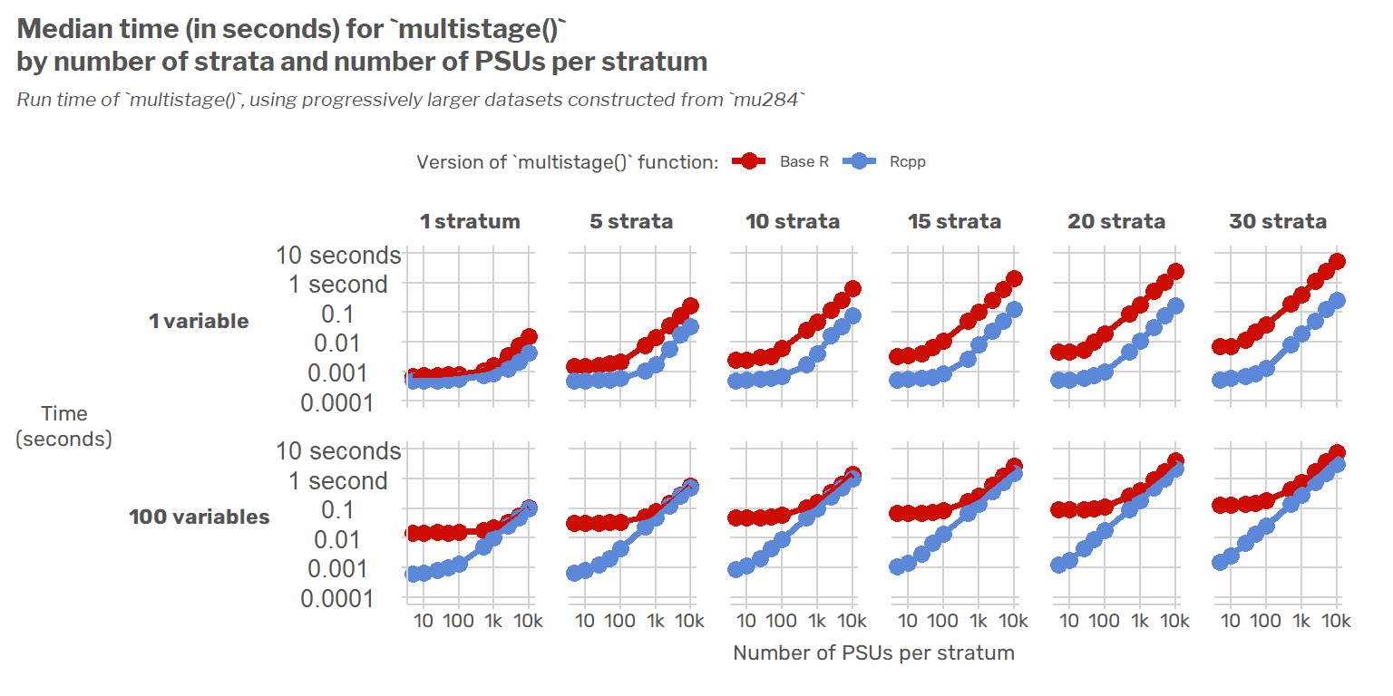
To motivate all this, I’ll start by showing speed benchmarks of the original functions and their {Rcpp} versions across a range of data sizes to understand when we should expect to see speed improvements. The TL;DR of this benchmarking is that the {Rcpp}-based functions are generally faster regardless of design size, and they scale much better as the number of PSUs or strata increases. The relative speed increase is much smaller though if a covariance matrix is being estimated for a large number of variables (say, 100).
Speed Benchmarking
Benchmarking the multistage() functions
To understand the relative speed performance of the base R and {Rcpp} versions of multistage(), I calculated the run time required to estimate the variance of a total for a range of different sizes of survey designs. The different sizes of survey designs I compared varied in terms of:
- The number of strata (1, 5, 10, 15, 20, 30)
- The number of PSUs per stratum (5, 10, 25, 50, 100, 500, 1,000, 2,500, 5,000, 10,000)
- The number of stages of sampling (1 or 2)
- The number of variables whose variances/covariances are to be estimated (1 or 100)
For each design size, I replicated the use of multistage() 30 times and calculated the median run time.
Click for code and more details about the benchmarking data
Datasets were constructing starting from the
mu284example dataset included in the {survey} package (type?mu284in R for details), which is an unstratified, two-stage sample with five PSUs and three SSUs within each PSU. To create larger designs, themu284dataset was duplicated as needed to create multiple strata and larger numbers of PSUs within each stratum. For example, to create a dataset with three strata and 10 PSUs per stratum, themu284dataset was duplicated six times, with each pair of duplicates grouped into different strata and the PSU ID labels updated to result in ten distinct PSUs per stratum.
Click to show R code for benchmarking
In the chart below, I show how the run times of the base R and {Rcpp} functions increase as the size of the survey design increases. The first chart (blue and red lines) shows the estimated run time in seconds for each function for single-stage designs, while the second chart shows the corresponding ratios of the function run times for both single-stage designs (blue) and two-stage designs (gold).
The {Rcpp} version of multistage() is generally always faster. As the number of strata increases, the {Rcpp} function increasingly performs much faster than its base R counterpart for any given number of PSUs per stratum. Once there are 10 or more strata, the {Rcpp} version is at least five times faster than the base R version for single-stage designs. For a large number of variables (100, say), the {Rcpp} function is much faster than its base R counterpart for a small number of PSUs per stratum, but the relative speed advantage of the {Rcpp} function declines as the number of PSUs per stratum increases.
For multistage designs, the {Rcpp} function can be several hundred times faster, even for a small number of strata and PSUs per stratum.
Note that this second chart is interactive and you can thus mouseover the datapoints for details.
Click to a view the table of data for this comparison
Adding unit tests for the new functions
Because this code would be used by producers of official statistics, it’s important to write unit tests that make sure it returns the expected results. Here, I describe an R script of unit tests I wrote for the new functions and how it fits into the existing suite of unit tests in the {survey} package.
The current suite of unit tests in the {survey} package
The {survey} package predates the rise of popular unit testing packages in R such as {testthat} or {tinytest}, but it has long had a suite of unit tests. The unit tests in the package are mostly structured as short scripts where a few examples of code are run to make sure that no error messages pop up when running a function and that the output can be manually inspected for correctness. For instance, here’s the unit test script for the workhorse multistage() function:
##
## Check that multistage samples still work
##
library(survey)
example(mu284)
And here are the first few lines of the unit test script for the handling of the survey.lonely.psu options:
## lonely PSUs by design
library(survey)
data(api)
## not certainty PSUs by fpc
ds<-svydesign(id = ~1, weights = ~pw, strata = ~dnum, data = apiclus1)
summary(ds)

options(survey.lonely.psu="fail")
try(svymean(~api00,ds))
try(svymean(~api00, as.svrepdesign(ds)))
options(survey.lonely.psu="remove")
svymean(~api00,ds)
svymean(~api00, as.svrepdesign(ds))
options(survey.lonely.psu="certainty")
svymean(~api00,ds)
svymean(~api00, as.svrepdesign(ds))
A notable feature of most of these tests is that they don’t compare the function results to an expected correct result. For example, a hypothetical function such as do_math <- function() {2 + 2} wouldn’t be checked to ensure that the output of do_math() equals 4. Rather, the user is simply able to view the output from calling do_math(), and the user can check for themselves that the result is correct. There are some important exceptions, such as the unit test for design effects in svyglm():
library(survey)

data(api)

## one-stage cluster sample
dclus1<-svydesign(id=~dnum, weights=~pw, data=apiclus1, fpc=~fpc)

# svyglm model
mod <- svyglm(api99 ~ enroll + api.stu, design = dclus1, deff = TRUE)

# run mod with same data and glm()
srs_mod <- glm(api99 ~ enroll + api.stu, data = apiclus1)

# manually calculate deffs

clust_se <- summary(mod)$coefficients[,2]
srs_se <- summary(srs_mod)$coefficients[,2]

deffs <- clust_se^2 / srs_se^2
stopifnot(all.equal(deffs, deff(mod)))
The new unit test script for the {Rcpp} Functions
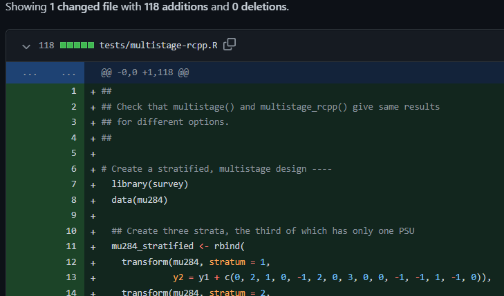
To test the {Rcpp}-based version of multistage(), I added the following file to the tests directory of the package.
The test script begins by checking whether multistage_rcpp() gives the same results as multistage() (the base R version) for a simple random sample example and for a stratified simple random sample. For the stratified SRS example, an additional check is added for whether the function returns “true zeroes” rather than infinitesimal nonzero numbers, as when the estimated totals are, say, the stratum population sizes.
Click for details about the check for “true zeroes”
The test for “true zeroes” was added because my experimentation found that there were tiny floating point differences (generally smaller than 1e-16 in absolute value) due to a slight difference in the precision of the C++ Armadillo sum() function compared to base R’s sum(). The {Rcpp} version of multistage() handles this issue at the end of its run by checking for variance estimates smaller than 1e-16 in absolute value and setting them (and their corresponding covariances) to 0.
See this bit of code:
// Deal with potential floating-point error
V.diag() = arma::abs(V.diag());
for (arma::uword i=0; i < V.n_cols; ++i ) {
  if (std::abs(V(i,i)) < 1e-16) {
    V.row(i).zeros();
    V.col(i).zeros();
  }
}
Additional tests are used to ensure correct handling under different settings related to singleton strata. The script sets up a handful of survey design objects with important features, such as the presence of strata with only a single PSU (i.e., “lonely PSUs”) caused by design or by subsetting to a domain with only one PSU. Then it sets up a grid of parameter and option settings (e.g., option(survey.lonely.psu = 'remove') with multistage(..., one.stage = TRUE)) and compares the {Rcpp} and base R versions of multistage() for each set of options. The key output is a dataframe with the list of options evaluated and a field named results_match indicating whether the base R and {Rcpp}-based functions returned the same results. If there are any mismatches, the script will throw an informative error message.
print(design_lonely_psu_comparisons)

#>   survey.lonely.psu one.stage results_match
#> 1         certainty      TRUE          TRUE
#> 2            remove      TRUE          TRUE
#> 3           average      TRUE          TRUE
#> 4            adjust      TRUE         FALSE
#> 5         certainty     FALSE          TRUE
#> 6            remove     FALSE          TRUE
#> 7           average     FALSE          TRUE
#> 8            adjust     FALSE         FALSE

if (!all(design_lonely_psu_comparisons$results_match)) {
    stop("Results for design lonely PSUs differ between base R and {Rcpp} implementations.")
}

#> Error: Results for design lonely PSUs differ between base R and {Rcpp} implementations.
#> Execution halted
In the current version of the {survey} package, the results match except when the user sets options(survey.lonely.psu = 'adjust'). However, this is because the {survey} package’s multistage() function has a long-standing bug in this case, as described in a recent blog post. and confirmed by email with Thomas. Unlike the base R version of multistage(), when the user sets options(survey.lonely.psu = 'adjust'), the lonely PSU gets recentered around the average PSU from across all strata (i.e., \(\hat{Y}/n\), where \(\hat{Y}\) is the vector of estimated totals and \(n\) is the number of PSUs from across all strata).
Adding the new {Rcpp} functions to the package
The GitHub repository “fastsurvey” (bschneidr/fastsurvey) is a fork of the {survey} package’s SVN repository on R-forge. The series of commits on the “adding-to-survey” branch shows the sequence of steps needed to add the Rcpp functions into the package, and I’ll outline them here.
Updating package files to allow Rcpp to be used
The first steps are generic package updates needed in order to allow {Rcpp} and the {RcppArmadillo} packages to be used.
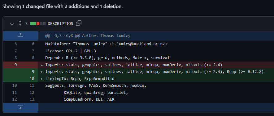
Step 1. Update DESCRIPTION file to use {Rcpp} and {RcppArmadillo} (click to view Git commit)
Step 2. Update NAMESPACE to use {Rcpp} (click to view Git commit)
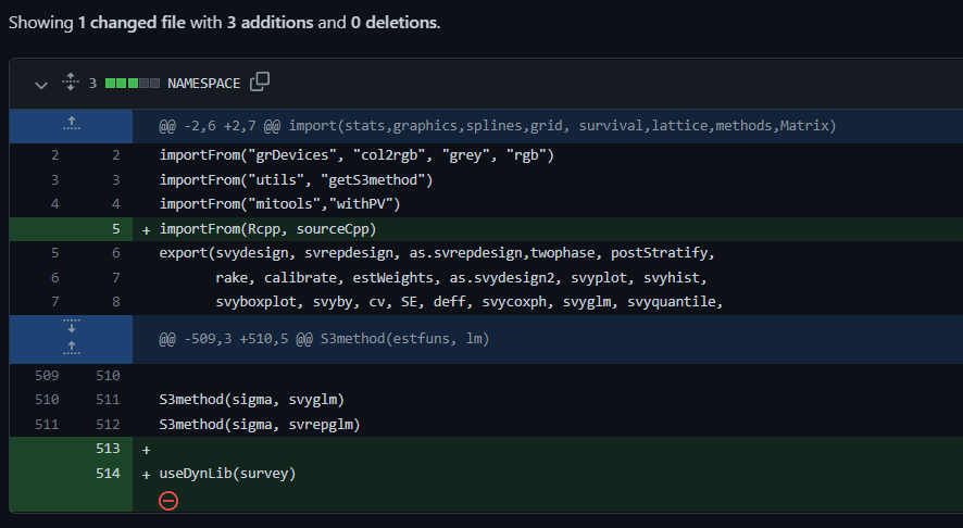
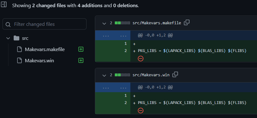
sourceCpp() is now imported from Rcpp, and the useDynLib(survey) line has been added.Step 3. Add necessary Makevars files for using {Rcpp} (click to view Git commit)
Adding the C++ functions
After the package has been set-up to allow the use of {Rcpp}, we add the “.cpp” source file for the new C++ functions used to do the intensive computations.
Step 4. Add “.cpp” file defining new Rcpp functions (click to view Git commit)
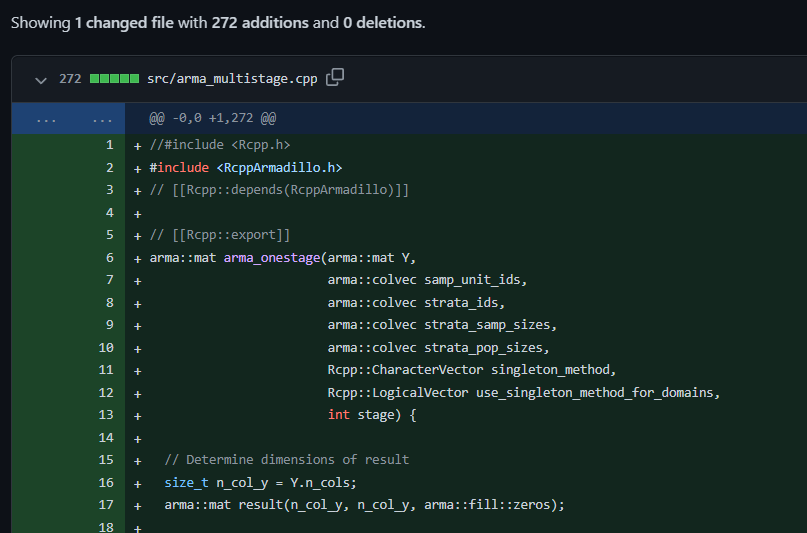
This “.cpp” file contains two functions. The function arma_onestage() calculates the variance of totals from a single stage of sampling (similar to survey:::onestage()), and the function arma_multistage() uses arma_onestage() as needed to calculate the variance of totals from multiple stages of sampling (similar to survey:::multistage()). These functions have very strict requirements for their input types and are purely for use internally in the package. They use the “arma_” prefix because they rely heavily on the {RcppArmadillo} package and we want to distinguish these functions from the existing R functions onestage() and multistage().
Step 5. Call Rcpp::compileAttributes() to export C++ functions for use in R. (click to view Git commit)
Once the package has been set up to use {Rcpp} and once we’ve added an actual “.cpp” file, we must run the R function Rcpp::compileAttributes() to generate files exporting the C++ functions for use in R. This step allows us to use the C++ functions as R functions. If we update the C++ code at any later point, we’ll need to rerun Rcpp::compileAttributes().
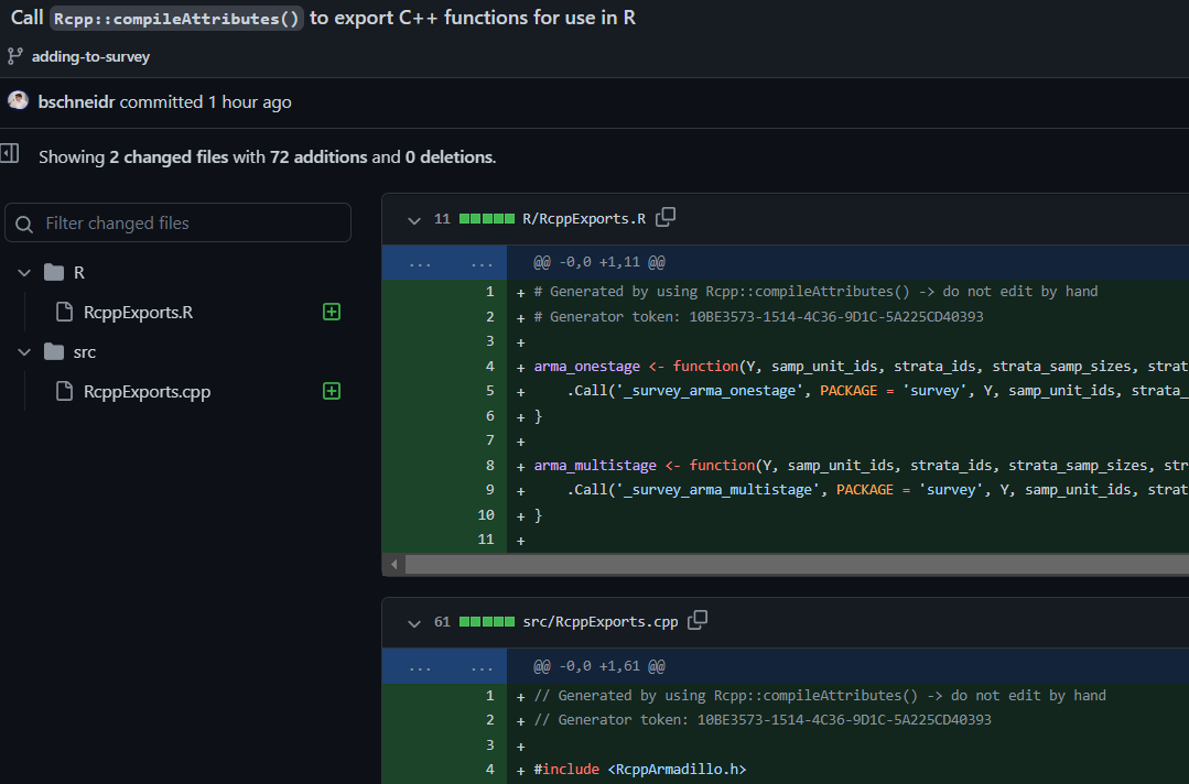
Rcpp::compileAttributes(). These files are named “R/RcppExports.R” and “src/RcppExports.cpp”. Both have the header text "Generated by using Rcpp::compileAttributes() -> do not edit by hand"Step 6. Add the the Rcpp-based version of multistage(), named multistage_rcpp(). (click to view Git commit)
At this point, we can call the arma_multistage() and arma_onestage() functions in R. However, since those are minimal wrappers around C++ code, they are very strict about the inputs they require. The key inputs (cluster IDs, strata IDs, etc.) must be numeric matrices, which is not a requirement of the original base R function multistage(). For that reason, I wrote the function multistage_rcpp() as a sort-of clone of multistage() that calls arma_multistage() after doing any necessary data type conversions to meet its strict input requirements.
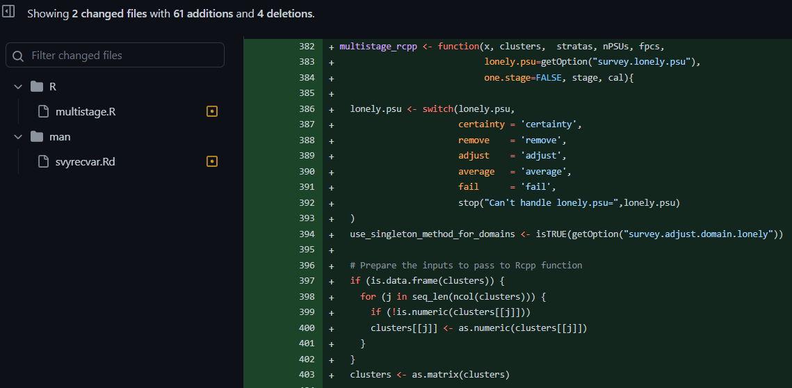
multistage_rcpp() added to the file “R/multistage.R” and the documentation file “man/svyrecvar.Rd” updated so that calling ?multistage_rcpp redirects to the same help page as calling ?svyrecvar.Step 7. Update svyrecvar() to use multistage_rcpp() where possible. (click to view Git commit)
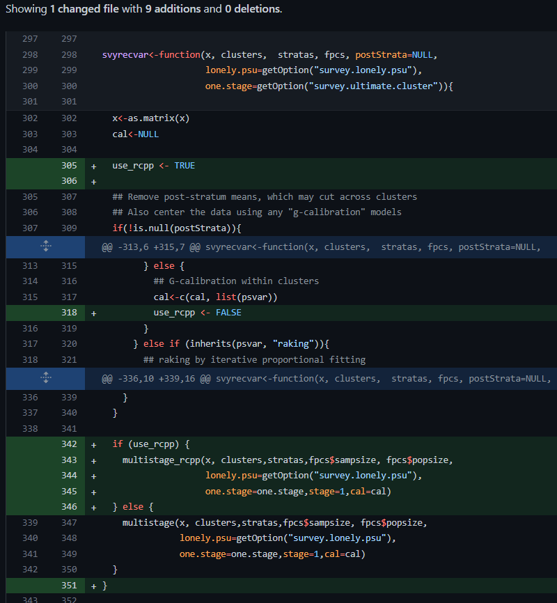
Finally, we’ll update svyrecvar() to use the faster multistage_rcpp() function whenever possible. Internally, the function svyrecvar() now has a flag named use_rcpp which is set to TRUE by default. However, if svyrecvar() detects that there has been any use of G-calibration within clusters (a fairly uncommon situation, I think), then it will set use_rcpp to FALSE and use the base R function multistage() instead of multistage_rcpp().
Click only if you want the tedious details about within-cluster G-calibration
The reason for switching is that the data structure used to represent within-cluster G-calibration is complex. Specifically, the survey design object’s postStrata element gets a list with identifiers for the cluster and its sampling stage, and an R object with class qr representing the QR-decomposition of the calibration variables.
For now, that’s too much of a headache for me to accommodate in the new functions, given that G-calibration within clusters is not something I ever see used (though it’s a good idea and I’m sure some R users are doing it). This certainly could be accomodated though, by updating the source code of the C++ functions in a few places and having multistage_rcpp() do a little more pre-processing of QR objects passed to it. The main headache is finding good example to use for development.
svyrecvar() to use the function multistage_rcpp() by default, and only use the base R function multistage() if there is G-calibration within clusters.Step 8: Adding unit tests (click to view Git commit)
Finally, we’ll add the script with unit tests. These tests compare the results of multistage_rcpp() to its base R equivalent multistage(), and throw an informative error message if there are any differences. As mentioned earlier, the only differences found in these unit tests at the moment are when the user sets option('survey.lonely.psu' = 'adjust').
Future work
Code Development
There are two cases where multistage_rcpp() isn’t currently able to replace base R counterparts.
Case 1. When there’s internal G-calibration within clusters. For this, I need a couple good examples to develop around and use for unit testing.
Case 2. For two-phase designs, the multistage.phase1() function is used to estimate sampling variance for the first stage. There’s not currently a multistage_rcpp.phase1() function developed, but it could certainly be done eventually.
I’d like to further develop the Rcpp/R code to cover those two cases, but I think their usage is uncommon enough that their development can wait until after the main {Rcpp} functions are added. It’s taken me easily more than a hundred hours to get the multistage_rcpp() function this far and to iron out all the issues uncovered during unit testing. The multistage_rcpp() function is ready for primetime, but it’s going to take a good bit longer to get the two other cases handled with C++ functions.
Dissemination
I think these faster C++ functions could be of interest to other survey-related packages. For example, the {rpms} package implemented its own C++ code to do fast variance estimation using the ultimate cluster approximation, but it could be helpful for it to instead rely on the {survey} package for its variance computations, which should now be at least as fast as the {rpms} variance estimation code but has the added advantages of being thoroughly unit-tested and useful for a wider variety of survey designs. After incorporating this into the {survey} package (or an add-on package, if necessary), it would be good to reach out to some package authors to let them know about the speed improvements.