Fitting a basic Fay-Herriot model in Stan and JAGS

Overview

This post builds on some of what I learned from the Small Area Estimation course at JPSM as well as a very interesting small area estimation project for work, which resulted in the recently-published paper with Westat colleagues Andreea Erciulescu and Jean Opsomer:

(Press Release) https://www.westat.com/articles/innovative-data-integration-methodology-developed-multilevel-modeling

(Paper) https://onlinelibrary.wiley.com/doi/10.1002/cjs.11688

For that project, we developed a model which is essentially a multivariate extension of the Fay-Herriot model, where some domains have unobserved values for one or more outcome variables. We first fit the model in JAGS, but we also tried using Stan in order to experiment with non-conjugate prior distributions for the variance components of the model. In this post, I share some of what I learned about fitting Bayesian Fay-Herriot models in JAGS and Stan, using publicly-available wage data from BLS for the purpose of illustration.

Our experience was that Stan and JAGS gave essentially the same results, and the alternative prior distribution had no real impact on our model inferences. However, Stan generally took much longer to obtain a sample of the same quality as what we were able to obtain with JAGS.

Background

The Fay-Herriot model is perhaps the most fundamental model in the field of small area estimation (SAE). The basic idea is simple. Suppose you want to estimate some quantity, such as the average wage, for each of several different cities, and you have only limited data from each city. To estimate an average wage for a given city in a given region, we have a couple of obvious options:

• The “direct estimate” approach. Produce a noisy estimate using just that city’s data. If the underlying sample data are representative and appropriate statistical procedures are used, then the estimates are unbiased but imprecise.

• The “completely pooled estimate”. Simply produce a single pooled estimate by aggregating together all of the estimates from cities in the region. Then use that as the estimate for each city in the region. Obviously this estimate is biased for each city (since cities should differ from one another), but the estimate is very precise and so might be better than the noisy estimate based on only the city’s data.

The Fay-Herriot model allows a compromise approach: for each city, use a weighted average of the city’s direct estimate and the regional average. For cities where the direct estimate is relatively precise (for example, if the sample size is large), assign more weight to the city’s direct estimate and less weight to the completely pooled region estimate. And in general, assign more weight to cities’ direct estimates if there appears to be large variation between cities. This strategy is referred to as “partial pooling”: estimates for a specific city are based on pooling together data from the specific city as well as other cities, but the city’s data is given more weight if it seems reliable.

In principle, this is an intuitive idea that probably feels like it’s just common sense. This is just a statistical way of saying the following:

“Consider the context. If a city’s noisy estimate is way higher than estimates from other similar cities, it’s probably an overestimate and we should adjust it to look more like the average city’s estimate.”

Of course, the devil is in the details.

Example data

For this example, we’ll use wage data published by the Bureau of Labor Statistics (BLS) as part of its Occupational Employment and Wage Statistics (OEWS) program. These data consist of estimated total employment and average wages in 2020 for hundreds of occupations in hundreds of metropolitan statistical areas (MSAs). Each estimate is accompanied with a standard error. ¹

We can get this data by downloading it as an Excel file from the BLS website.²

# Download the '.zip' file from BLS and extract the Excel file
bls_data_link <- "https://www.bls.gov/oes/special.requests/oesm20ma.zip"
temp_zip_file <- tempfile(fileext = ".zip")
temp_data_folder <- tempdir()

download.file(url = bls_data_link, destfile = temp_zip_file)
unzip(zipfile = temp_zip_file,
      exdir = temp_data_folder,
      files = "oesm20ma/MSA_M2020_dl.xlsx")

# Read in the data from the Excel file
raw_msa_data <- readxl::read_xlsx(path = file.path(temp_data_folder, "oesm20ma",
                                               "MSA_M2020_dl.xlsx"),
                              sheet = "MSA_M2020_dl")

# Delete the downloaded data files
unlink(temp_zip_file)
unlink(temp_data_folder)

library(dplyr)

msa_data <- raw_msa_data %>%
  select(
    # MSA name and code
    AREA, AREA_TITLE, 
    # Occupation name and code
    O_GROUP, OCC_CODE, OCC_TITLE, 
    # Employment estimate, and its std. error
    TOT_EMP, EMP_PRSE, 
    # Mean annual wage estimate, and its std. error
    A_MEAN_WAGE = A_MEAN, A_MEAN_WAGE_PRSE = MEAN_PRSE 
  ) %>%
  # Ensure variables are stored as numeric
  # and standard errors are on the same scale as the estimate
  mutate(across(matches("EMP|MEAN"), as.numeric)) %>%
  mutate(TOT_EMP_SE = (EMP_PRSE/100) * TOT_EMP,
         A_MEAN_WAGE_SE = (A_MEAN_WAGE_PRSE/100) * A_MEAN_WAGE) %>%
  select(-EMP_PRSE, -A_MEAN_WAGE_PRSE) %>%
  # Rearrange columns for ease of reading
  select(matches("AREA"), starts_with("O"),
         starts_with("TOT_EMP"), starts_with("A_MEAN_WAGE"))

knitr::kable(head(msa_data, 5))

AREA	AREA_TITLE	O_GROUP	OCC_CODE	OCC_TITLE	TOT_EMP	TOT_EMP_SE	A_MEAN_WAGE	A_MEAN_WAGE_SE
10180	Abilene, TX	total	00-0000	All Occupations	66060	1255.14	42930	772.74
10180	Abilene, TX	major	11-0000	Management Occupations	2910	130.95	89160	1961.52
10180	Abilene, TX	detailed	11-1021	General and Operations Managers	1320	97.68	83990	2939.65
10180	Abilene, TX	detailed	11-2022	Sales Managers	90	16.65	121020	9197.52
10180	Abilene, TX	detailed	11-2030	Public Relations and Fundraising Managers	40	12.60	95540	19776.78

For context, the estimates are available for occupations within metropolitan statistical areas (MSAs), and occupations are defined at both a detailed level (a six-digit code known as an SOC6) and a major level (a two-digit code known as an SOC2), where detailed SOC6 occupations are nested within major SOC2 occupations. This suggests that if we’re interested in estimates for detailed occupations in MSAs, we can improve our estimates by pooling across MSAs within a region and/or by pooling across detailed SOC6 occupations within a major SOC2 occupation.

Inspect the data

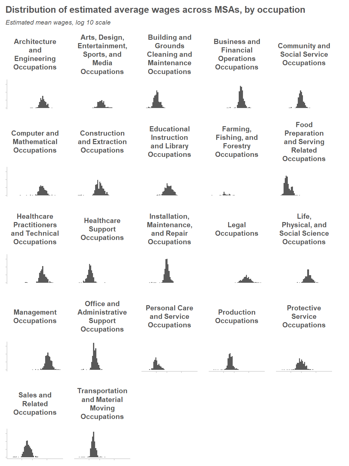
Let’s take a look at the distribution of wage estimates across MSAs, within each major occupation group. We’ll focus on the MSAs where the estimates appear to be relatively precise (i.e. where the estimated percent relative standard error is under 10%); this will allow us to get a sense of what the actual variability across MSAs looks like. At a first glance, it looks like a log-normal distribution would provide a reasonable model of variability across MSAs.

Warning: Ignoring unknown parameters: labels

Warning: Removed 38 rows containing non-finite values (stat_bin).

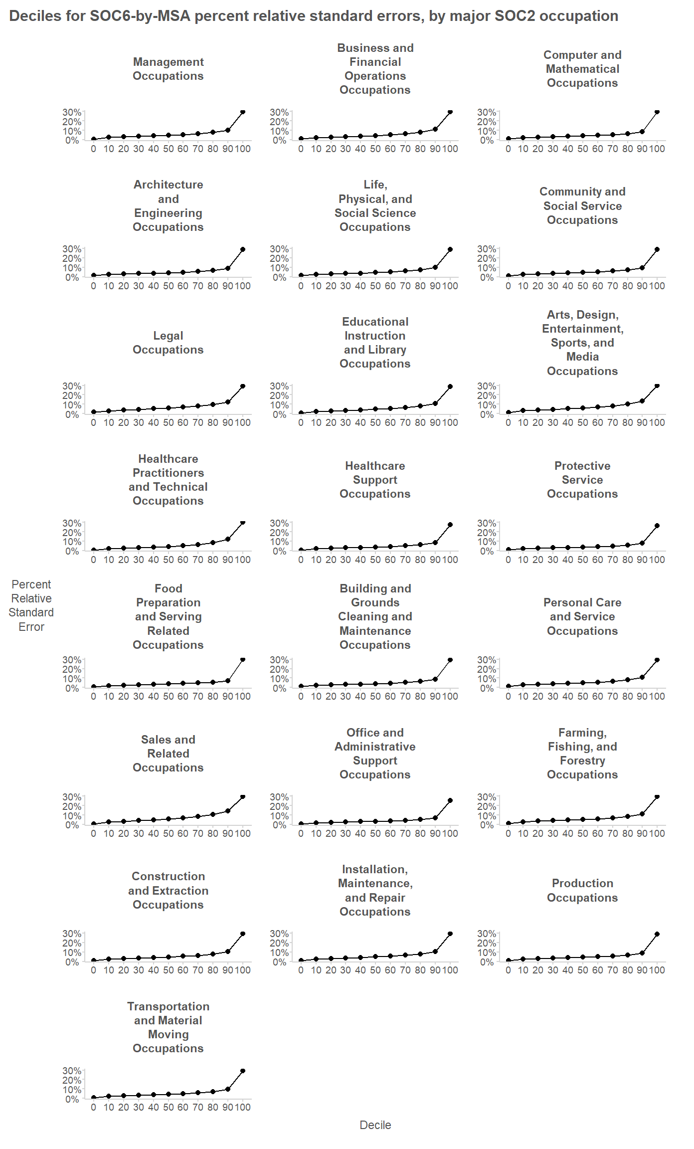
Next we’ll try to see how (im)precise the detailed occupational wage estimates are.

AREA_TITLE	MAJOR_OCC	OCC_TITLE	A_MEAN_WAGE	A_MEAN_WAGE_SE
Abilene, TX	Management Occupations	General and Operations Managers	83990	2939.65
Abilene, TX	Management Occupations	Sales Managers	121020	9197.52

From the plot, it is apparent that the PRSEs are all below 30%. This reflects BLS publication standards preventing the publication of highly imprecise estimates; estimates whose PRSE are above 30% are generally not published. The 90% quantiles for the PRSEs are generally between 8% and 14%.

`summarise()` has grouped output by 'SOC2', 'MAJOR_OCC'. You can override using
the `.groups` argument.

Fit a basic model

For both Stan and JAGS, we have to write our model using special language. This written model can be passed to Stan/JAGS either as a string in R (e.g. "y ~ normal(0, 1)") or by supplying a standalone file saved on your computer. Below we’ll write out our model in mathematical notation and in the special modeling languages for Stan and for JAGS.

The average annual wage for a given domain (i.e. a given occupation in a given city) is denoted \(\theta_j\). The direct estimate based on survey data from just that domain is \(\hat{\theta}_j\), and its sampling variance is \(V_j\).

Because the variation in average wages across domains seems to follow a log-normal distribution, we’ll model the log-transformed parameter, \(\theta_{j,log}=ln(\theta_j)\) and its estimate \(\hat{\theta}_{j,log}=log(\hat{\theta_j})\). To obtain the sampling variance of \(\hat{\theta}_{j,log}=log(\hat{\theta_j})\), we’ll use the Delta Method: \(V_{j,log} := \frac{1}{(\hat{\theta})^2}V_j\). Note that \(V_{j,log}\) is an estimate (and so is \(V_j\)), but for modeling purposes we ignore that fact and assume that these are known values. This assumption can be relaxed but we’ll avoid getting into the complicated variance modeling required to do so.

The log-normal distribution is commonly-used in economics to model wage and income distributions, and there has been much theoretical work done in economics to understand why this distribution often provides a good description of wage/income distributions.

\[ \begin{aligned} \\ \underline{\textbf{Sampling }\textbf{Level}}& \\ \textbf{Likelihood}& \\ \hat{\theta}_{j,log} &\sim {N}\left(\theta_{j,log},V_{j,log}\right) \\ \underline{\textbf{Smoothing }\textbf{Level}}& \\ \textbf{Likelihood}& \\ \theta_{j,log} &\sim {N}\left(\mu,\sigma^2\right) \\ \textbf{Priors}& \\ \mu &\sim {N}\left(\ln(50,000), \ln(50,000)^2 \space\right) \\ \sigma^2 &\sim \text{Inv-Gamma}\left(0.001, 0.001\right) \end{aligned} \]

Loading required package: coda

Linked to JAGS 4.3.1

Loaded modules: basemod,bugs

Loading required package: StanHeaders

rstan (Version 2.21.5, GitRev: 2e1f913d3ca3)

For execution on a local, multicore CPU with excess RAM we recommend calling
options(mc.cores = parallel::detectCores()).
To avoid recompilation of unchanged Stan programs, we recommend calling
rstan_options(auto_write = TRUE)

Do not specify '-march=native' in 'LOCAL_CPPFLAGS' or a Makevars file

Attaching package: 'rstan'

The following object is masked from 'package:coda':

    traceplot

Stan Model Syntax

data {
  int<lower=0> J;
  real dir_est[J];
  real<lower=0> dir_est_std_error[J];
}
parameters {
  real theta[J];
  real mu;
  real<lower=0> sigma2;
}
model {
  // Likelihood
    //-- Sampling level
    dir_est ~ normal(theta, dir_est_std_error) ;
    //-- Smoothing level
    theta ~ normal(mu, sqrt(sigma2)) ;
  // Priors
    //-- Uninformative prior on variance of distribution
    sigma2 ~ inv_gamma(0.001, 0.001);
    //-- Weakly informative prior on center of distribution
    mu ~ normal(log(50000),log(50000))
}

JAGS Model Syntax

model {
# Likelihood
  for (j in 1:J) {
    dir_est_precision[j] <- 1/dir_est_std_error[j]^2
    dir_est[j] ~ dnorm(theta[j], dir_est_precision[j])
    theta[j] ~ dnorm(mu, inv_sigma2)
  }
# Priors
  ## Uninformative prior on variance of distribution
  inv_sigma2 ~ dgamma(0.001, 0.001)
  sigma2 <- 1/inv_sigma2
  ## Weakly informative prior on center of distribution
  mu ~ dnorm(log(50000), log(50000))
}

How were those priors chosen? For the prior on \(\sigma^2\), I used a common uninformative prior for the variance of a Normal distribution. The Inverse-Gamma distribution is a conjugate prior for this case, and so it can be used in both Stan and JAGS.

For the prior on \(\mu\), I wanted a weakly informative prior and so I chose a Normal prior that, on the non-logarithmic scale, is centered at right about the average annual wage for the U.S. overall, and which is diffuse in the sense that it has a coefficient of variation of 100%. The reason for using a weakly-informative prior in this case is that we do have good external information about the center of the wage distribution which we can easily incorporate into our model, and doing so may slightly improve the precision of our estimates.

Using JAGS

We’ll fit this basic model in JAGS first. The input data needs to be an R list object, with elements whose names match the data described in our JAGS model.

# Prepare the data for JAGS ----
model_data <- msa_by_soc6_data[,c("AREA_TITLE", "OCC_TITLE",
                                  "A_MEAN_WAGE", "A_MEAN_WAGE_SE")] %>%
  na.omit()

model_input_data <- list(
  J = nrow(model_data),
  dir_est = log(model_data$A_MEAN_WAGE),
  dir_est_std_error = (1/model_data$A_MEAN_WAGE) * model_data$A_MEAN_WAGE_SE
)

# Prepare the model for MCMC sampling ----
jags_fh_model <- rjags::jags.model(
  data = model_input_data,
  file = textConnection(
"model {
# Likelihood
  for (j in 1:J) {
    dir_est_precision[j] <- 1/dir_est_std_error[j]^2
    dir_est[j] ~ dnorm(theta[j], dir_est_precision[j])
    theta[j] ~ dnorm(mu, inv_sigma2)
  }
# Priors
  ## Uninformative prior on variance of distribution
  inv_sigma2 ~ dgamma(0.001, 0.001)
  sigma2 <- 1/inv_sigma2
  ## Weakly informative prior on center of distribution
  mu ~ dnorm(log(50000), log(50000))
}"
),
  n.chains = 2
)

Compiling model graph
   Resolving undeclared variables
   Allocating nodes
Graph information:
   Observed stochastic nodes: 127833
   Unobserved stochastic nodes: 127835
   Total graph size: 384096

Initializing model

After declaring the model, we use the update() function to “burn-in” a desired number of iterations.

update(jags_fh_model, n.iter = 1000)

Then we can use the code.samples() function to draw a sample with a desired thinning rate. By using the variable.names argument, we can control which variables to retain in our output of posterior draws; this can be useful if there are many nuisance parameters.

A Note on Thinning

While thinning is counterproductive in many (if not most) cases, it is in fact helpful here. Despite the popular misconception that thinning is necessary for MCMC inference, the decision to use a thinned chain almost always worsens the quality of our estimates compared to using an unthinned chain (see Link and Eaton 2010), as we are reducing our Monte Carlo sample size. However, thinning increases the information content of data of a given size. So when our model is large (as in our example, with its 100,000+ parameters of interest) and our ability to store the posterior draws and work with them is limited by memory/computational constraints, thinning gets us more value from our costly storage and computations.

# Draw MCMC samples ----
## Run the chain for 5,000 iterations,
## retaining every 10th iteration

jags_posterior_samples <- coda.samples(
  model = jags_fh_model, n.iter = 5000, thin = 10,
  variable.names = c('theta', 'mu', 'sigma2')
)

Let’s examine the output from the samples. We can obtain a neat data frame of results using the tidy_draws() function from the handy {tidybayes} R package: one row per draw per chain, and one column per parameter of interest.

tidy_jags_samples <- tidybayes::tidy_draws(model = jags_posterior_samples)
str(tidy_jags_samples[,1:10])

tibble [1,000 × 10] (S3: tbl_df/tbl/data.frame)
 $ .chain    : int [1:1000] 1 1 1 1 1 1 1 1 1 1 ...
 $ .iteration: int [1:1000] 1 2 3 4 5 6 7 8 9 10 ...
 $ .draw     : int [1:1000] 1 2 3 4 5 6 7 8 9 10 ...
 $ mu        : num [1:1000] 10.8 10.8 10.8 10.8 10.8 ...
 $ sigma2    : num [1:1000] 0.22 0.219 0.22 0.219 0.221 ...
 $ theta[1]  : num [1:1000] 11.3 11.3 11.4 11.3 11.3 ...
 $ theta[2]  : num [1:1000] 11.6 11.7 11.8 11.8 11.6 ...
 $ theta[3]  : num [1:1000] 11.1 11.4 11.3 11.3 11.1 ...
 $ theta[4]  : num [1:1000] 11.2 11.3 11.3 11.2 11.2 ...
 $ theta[5]  : num [1:1000] 11.7 11.8 11.7 11.7 11.8 ...

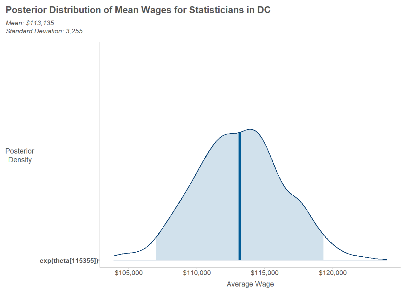
To summarize the posterior draws for a given parameter, we simply work with the rows for a column of interest. For illustration, we’ll look at the posterior distribution for average wages among statisticians in D.C.

# Determine name of the parameter ----
j_dc_statistician <- model_data %>%
  mutate(j = row_number()) %>%
  filter(stringr::str_detect(OCC_TITLE, "Statistician"),
         stringr::str_detect(AREA_TITLE, "Washington.+DC")) %>%
  pull("j")

print(j_dc_statistician)

[1] 115355

param_of_interest <- sprintf("theta[%s]", j_dc_statistician)
print(param_of_interest)

[1] "theta[115355]"

# Extract posterior draws and exponentiate
# (since the model is specified on the log scale)
param_samples <- exp(tidy_jags_samples[[param_of_interest]])

# Calculate summaries of interest (mean and standard deviation)
post_mean <- mean(param_samples)
post_sd <- sd(param_samples)

# Format summaries into text
text_summary <- sprintf(
  "Mean: %s\nStandard Deviation: %s",
  mean(exp(tidy_jags_samples[[param_of_interest]])) %>%
    scales::dollar(),
  sd(exp(tidy_jags_samples[[param_of_interest]])) %>%
    scales::comma()
)

writeLines(text_summary)

Mean: $113,213
Standard Deviation: 3,196

To visualize the posterior sample, we can use the handy mcmc_areas() function from the {bayesplot} package.

library(bayesplot)

This is bayesplot version 1.9.0

- Online documentation and vignettes at mc-stan.org/bayesplot

- bayesplot theme set to bayesplot::theme_default()

   * Does _not_ affect other ggplot2 plots

   * See ?bayesplot_theme_set for details on theme setting

mcmc_areas(jags_posterior_samples,
           pars = param_of_interest,
           transformations = "exp", prob = 0.95) +
  scale_x_continuous(labels = scales::dollar) +
  labs(
    title = "Posterior Distribution of Mean Wages for Statisticians in DC",
    x = "Average Wage",
    y = "Posterior\nDensity",
    subtitle = text_summary
  )

Scale for 'x' is already present. Adding another scale for 'x', which will
replace the existing scale.

Using Stan

Now let’s fit the same model using Stan. There are a couple of different packages we can use–{rstan} or the in-development {cmdstanr}–but here we’ll stick with {rstan} because it’s more stable and better documented.

First, we write out our model in Stan code, either as a ‘.stan’ file or as a character string. Because our model is fairly small, we’ll use a character string for the sake of illustration. Then we supply the model and our data to the function stan(). Note that we can use the exact same input data for Stan here as we used for JAGS.

model_code <- 
"data {
  int<lower=0> J;
  real dir_est[J];
  real<lower=0> dir_est_std_error[J];
}
parameters {
  real theta[J];
  real mu;
  real<lower=0> sigma2;
}
model {
  // Likelihood
    //-- Sampling level
    dir_est ~ normal(theta, dir_est_std_error) ;
    //-- Smoothing level
    theta ~ normal(mu, sqrt(sigma2)) ;
  // Priors
    //-- Uninformative prior on variance of distribution
    sigma2 ~ inv_gamma(0.001, 0.001);
    //-- Weakly informative prior on center of distribution
    mu ~ normal(log(50000),log(50000));
}"

library(rstan)

stan_fit <- stan(
  model_code = model_code,  # Stan program
  data = model_input_data,  # named list of data
  chains = 2,               # number of Markov chains
  warmup = 1000,            # number of warmup iterations per chain
  iter = 6000,              # total number of iterations per chain (incl. warmup)
  thin = 10,                # thinning interval
  cores = 2,                # number of cores (could use one per chain)
  refresh = 500             # refresh progress bar every 500 iterations
)

This model took much longer to fit in Stan than in JAGS (10 minutes versus two hours). For the same amount of computational time required to use Stan here, we could have used JAGS to run more chains for more iterations. However, some benefits of the Stan model include more built-in MCMC diagnostics and, if we had chosen, better ability to handle non-conjugate prior distributions.

Just like we did with the JAGS output, we can use the {tidybayes} package to obtain a tidy data frame of the posterior draws.

tidy_stan_samples <- tidybayes::tidy_draws(model = stan_fit)
str(tidy_stan_samples[,1:10])

tibble [800 × 10] (S3: tbl_df/tbl/data.frame)
 $ .chain    : int [1:800] 1 1 1 1 1 1 1 1 1 1 ...
 $ .iteration: int [1:800] 1 2 3 4 5 6 7 8 9 10 ...
 $ .draw     : int [1:800] 1 2 3 4 5 6 7 8 9 10 ...
 $ theta[1]  : num [1:800] 11.3 11.3 11.3 11.3 11.4 ...
 $ theta[2]  : num [1:800] 11.6 11.7 11.8 11.7 11.7 ...
 $ theta[3]  : num [1:800] 11.1 11.1 11.3 11 11.4 ...
 $ theta[4]  : num [1:800] 11.3 11.3 11.3 11.3 11.2 ...
 $ theta[5]  : num [1:800] 11.8 11.6 11.6 11.7 11.7 ...
 $ theta[6]  : num [1:800] 11.7 11.6 11.6 11.7 11.7 ...
 $ theta[7]  : num [1:800] 11.7 11.4 11.6 11.5 11.7 ...

Comparing Stan and JAGS Fits

With the tidied outputs in hand, we can compare the posterior estimates from Stan and JAGS. First, we’ll create a data frame with the original estimates side-by-side with the posterior means and standard deviations from both of the two pieces of software.

# A tibble: 6 × 8
  AREA_TITLE  OCC_TITLE A_MEAN_WAGE A_MEAN_WAGE_SE POST_MEAN_STAN POST_MEAN_JAGS
  <chr>       <chr>           <dbl>          <dbl>          <dbl>          <dbl>
1 Abilene, TX General …       83990          2940.         83886.         83724.
2 Abilene, TX Sales Ma…      121020          9198.        118865.        118941.
3 Abilene, TX Public R…       95540         19777.         86303.         87670.
4 Abilene, TX Administ…       78600          2751          78416.         78478.
5 Abilene, TX Computer…      123040         10458.        119463.        120226.
6 Abilene, TX Financia…      119580         11480.        115419.        116467.
# … with 2 more variables: POST_SD_STAN <dbl>, POST_SD_JAGS <dbl>

Let’s see whether the Stan and JAGS estimates are similar (as we’d hope). The correlation is nearly 1.0 and, the relative difference in the domain estimates rarely exceeds 1% and never exceeds 4%.

[1] 0.9999732

[1] 0.9988437

In short, the estimates from fitting this model in Stan vs. JAGS are essentially the same. But there are some small discrepancies likely attributable to random variation that occurs in any MCMC simulation, and so we would want to increase the number of draws if we were actually going to publish or otherwise act upon these estimates.

Evaluating the Pooling Induced by the Fay-Herriot Model

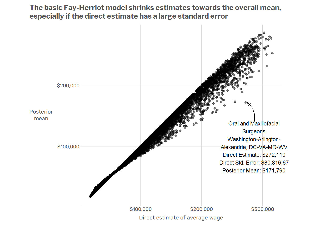
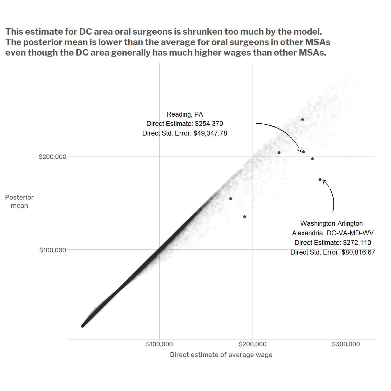
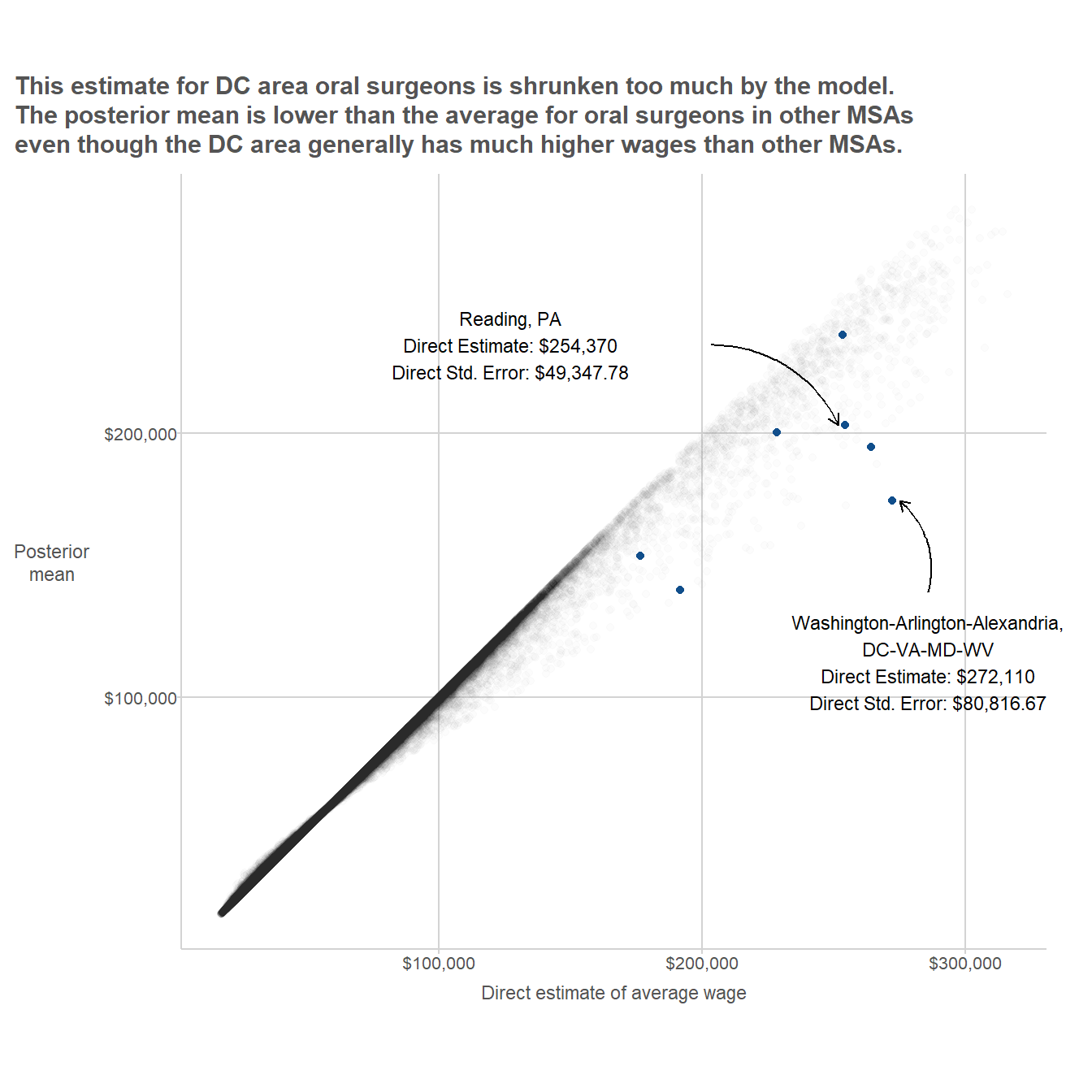
Next we can plot the original direct estimates against the estimates from the Fay-Herriot model. For the sake of illustration, we can highlight one particular domain where there is a large difference between the original direct estimate and the posterior mean from the Fay-Herriot model.

Registering fonts with R

Some Potential Improvements for the Model

This basic model has a couple of obvious issues. For starters, it ignores big, systematic patterns of variation in the data. Wages vary dramatically across regions and across major SOC2 groups. For example, the average wage in the D.C. metro area is about $10/hour higher than in Miami, and occupations in the “Food Preparation and Serving” SOC2 group usually have lower wages than occupations in the “Healthcare Practitioners and Technical Occupations” SOC2 group. But when the model produces estimates for oral surgeons in the Washington D.C. MSA, it is just as influenced by data from waiters in Miami as by data from nurses in Virginia or Maryland. This results in model-induced mistakes such as that illustrated in the plot below, which shows that

A better model would make use of the fact that when estimating wages for oral surgeons, the data on nurses in the same state are more relevant than data from non-medical professions in other states. One way to do this would be to add random effects for geographic areas (MSAs, states, or some combination thereof) and occupations (at the SOC2 or perhaps SOC6 level). That’s the approach that Andreea, Jean, and I took in the paper mentioned at the beginning of this post.

Footnotes

1. The data file represents standard errors as a “percent relative standard error (PRSE)”, which is the ratio of an estimate’s standard error to the estimate itself, expressed as a percentage.

2. There are actually multiple fine R packages for downloading BLS data, I just don’t have the motivation to figure out which one to use or how to use it.