set.seed(1999)

# Set the population size
N <- 50000

# Generate ages
ages <- runif(n = N, min = 18, max = 65)
ages <- round(ages)

# Generate vaccination status
random_component <- rnorm(n = N, mean = 0, sd = 1)

vaxxed_prob <- plogis(
  ( (1/3) * scale(ages, center = TRUE, scale = TRUE)  )
  +
  ( (2/3) * (0.5 + random_component))
)
vaxxed <- ifelse(vaxxed_prob > 0.5, 1, 0)

pop <- data.frame(
  'Person' = 1:N,
  'Age' = ages,
  'Vaxxed' = vaxxed
)The problem
Suppose we have a survey of adults which measures Covid-19 vaccination status. Now suppose we want to estimate the vaccination rate \(R\) of two overlapping populations: persons aged 30-50 years old and persons aged 40-60 years old. We’ll denote our two vaccination rates \(R_1\) and \(R_2\). It’s straightforward to estimate the sampling variance of each statistic, \(Var(\hat{R}_1)\) and \(Var(\hat{R}_2)\), separately.
But if we want to estimate the sampling variance of, say, the estimated difference in vaccination rates, \(R_1 - R_2\), we need to know the covariance/correlation of the two estimates \(\operatorname{Cov}(\hat{R_1},\hat{R_2})\). If the two groups were totally distinct, we might be able to assume that this correlation is zero. But since the two groups overlap, their estimates are almost certainly correlated. So how do we estimate this correlation?
In other words, how do we estimate the covariance of statistics from overlapping subsets of our sample?
Influence functions to the rescue
In a recent post, we saw how the survey package in R uses influence functions to estimate variances for non-overlapping domains, such as elementary schools and middle schools. But influence functions can also be used to estimate variances for overlapping domains!
Background on the influence function method for a single statistic’s variance
Many population quantities of interest (means, ratios, regression coefficients, Gini coefficients, etc.) can in a sense be approximated by their influence functions, which are defined for each person \(i\) in the population and are denoted \(z_i\). For example, for a population mean \(\bar{Y}\), the influence function for person \(i\) is \(z_i=\frac{1}{N}(y_i - \bar{Y})\).
To estimate the sampling variance of a statistic used to estimate the parameter (e.g. a mean \(\hat{\bar{Y}}\) or a ratio \(\hat{R}=\hat{Y}/{\hat{X}}\)), we can instead estimate the sampling variance of the statistic \(\hat{Z}=\sum_{i \in s} w_iz_i\), which is simply an estimated population total. 1 This is useful because for any common survey design (cluster sampling, PPS sampling, etc.), it’s easy to estimate population totals and their sampling variances. What’s more, the influence functions are population values that do not depend on the sample. Thus, the influence function method allows us to take a hard problem–estimating the variance of a complicated statistic–and turn it into an easier problem: estimating the variance of an estimated population total.
Using influence functions for covariances
Now suppose we have two population quantites, such as the vaccination rate for adults aged 30-50, denoted \(\bar{R}_1\), and the estimated vaccination rate for adults aged 40-60, denoted \(\bar{R}_2\). Both of these quantities are means, which we can write as follows:
\[ \begin{aligned} y_i &= \begin{cases}1~&{\text{ if person }}i~\text{is vaccinated}~\\0~&{\text{ if person }}i~\text{is unvaccinated}~.\end{cases} \\ d_{1,i} &= \begin{cases}1~&{\text{ if person }}i~\text{is aged 30-50}~\\0~&{\text{ otherwise}}~\end{cases} \\ d_{2,i} &= \begin{cases}1~&{\text{ if person }}i~\text{is aged 40-60}~\\0~&{\text{ otherwise}}~\end{cases} \\ \\ y_{1,i} &= y_i \times d_{1,i} \\ y_{2,i} &= y_i \times d_{2,i} \\ \\ N_1 &= \sum_{i=1}^{N} d_{1,i} \\ N_2 &= \sum_{i=1}^{N} d_{2,i} \\ \\ \bar{R}_1 &= \frac{1}{N_1} \sum_{i=1}^{N}y_{1,i} \\ \bar{R}_2 &= \frac{1}{N_2} \sum_{i=1}^{N}y_{2,i} \\ \end{aligned} \]
Both of these population quantities have influence functions, which are as follows:
\[ \begin{aligned} z_{1,i} &= \frac{1}{N_1}(y_{1,i} - R_1 \times d_{1,i}) \\ z_{2,i} &= \frac{1}{N_2}(y_{2,i} - R_2 \times d_{2,i}) \\ \end{aligned} \]
Have you guessed yet what we’re going to do?
That’s right: we’ll estimate the covariance of the estimated totals \(\hat{Z}_1=\sum_{i \in s} w_i z_{1,i}\) and \(\hat{Z}_2=\sum_{i \in s} w_i z_{2,i}\).
Well, almost. Since the influence functions \(z_{1,i}\) and \(z_{2,i}\) depend on unknown population quantities \(R_1,R_2\) and \(N_1,N_2\), we’ll estimate those first and then “plug in” those quantities to the formulas above in order to get estimated influence functions, \(\tilde{z}_{1,i}\) and \(\tilde{z}_{2,i}\). Then we’ll estimate the covariance of the statistics \(\tilde{Z}_1=\sum_{i \in s} w_i \tilde{z}_{1,i}\) and \(\tilde{Z}_2=\sum_{i \in s} w_i \tilde{z}_{2,i}\). In short, we’ll make the following approximation:
\[ \begin{aligned} Cov(\hat{R}_1, \hat{R}_2) &\approx Cov(\tilde{Z}_1,\tilde{Z}_2) \\ \text{where}& \\ \tilde{Z}_1&=\sum_{i \in s} w_i \tilde{z}_{1,i} \\ \tilde{Z}_2 &= \sum_{i \in s} w_i \tilde{z}_{2,i} \\ \text{and } \\ \tilde{z}_{1,i} &= \frac{1}{\hat{N}_1}(y_{1,i} - \hat{R}_1 \times d_{1,i}) \\ \tilde{z}_{2,i} &= \frac{1}{\hat{N}_2}(y_{2,i} - \hat{R}_2 \times d_{2,i}) \\ \end{aligned} \]
An example with the survey R package
Simulating a population
To illustrate how this works, we’ll simulate an artificial population where about 67% of the population is vaccinated, and age accounts for about 1/3 of the variation in vaccination status. The R code is shown below.
Here’s what the data for the population looks like:
# A tibble: 10 × 3
   Person   Age Vaxxed
    <int> <dbl>  <dbl>
 1      1    54      1
 2      2    43      0
 3      3    41      1
 4      4    37      0
 5      5    60      1
 6      6    43      1
 7      7    62      1
 8      8    51      1
 9      9    44      0
10     10    58      1
Next we’ll add variables that define the domains of interest:
# Calculate indicators for age category
pop[['Aged_30_to_50']] <- ifelse(
  (pop$Age >= 30 & pop$Age <= 50),
  1, 0
)
pop[['Aged_40_to_60']] <- ifelse(
  (pop$Age >= 40 & pop$Age <= 60),
  1, 0
)

# Calculate indicators for vaccination status by age category
pop[['Vaxxed_30_to_50']] <- pop$Vaxxed * pop$Aged_30_to_50
pop[['Vaxxed_40_to_60']] <- pop$Vaxxed * pop$Aged_40_to_60
# A tibble: 10 × 7
Person Age Vaxxed Aged_30_to_50 Aged_40_to_60 Vaxxed_30_to_50
<int> <dbl> <dbl> <dbl> <dbl> <dbl>
1 1 54 1 0 1 0
2 2 43 0 1 1 0
3 3 41 1 1 1 1
4 4 37 0 1 0 0
5 5 60 1 0 1 0
6 6 43 1 1 1 1
7 7 62 1 0 0 0
8 8 51 1 0 1 0
9 9 44 0 1 1 0
10 10 58 1 0 1 0
# ℹ 1 more variable: Vaxxed_40_to_60 <dbl>Now we can calculate the population vaccination rates as follows:
# Calculate population vaccination rates

  ##_ First for population aged 30 to 50
  N_30_to_50 <- sum(pop$Aged_30_to_50)
  Y_30_to_50 <- sum(pop$Vaxxed_30_to_50)

  R_30_to_50 <- Y_30_to_50 / N_30_to_50

  ##_ Next for population aged 40 to 60
  N_40_to_60 <- sum(pop$Aged_40_to_60)
  Y_40_to_60 <- sum(pop$Vaxxed_40_to_60)

  R_40_to_60 <- Y_40_to_60 / N_40_to_60
Summarized in a plot:
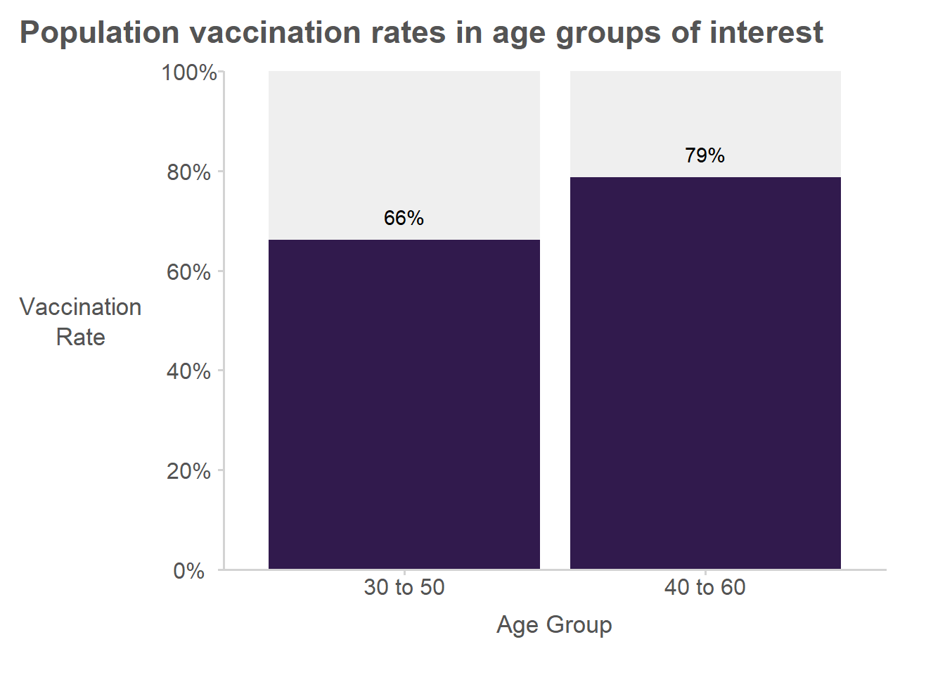
Summarized in a table:
| Age Group | Size | Total Vaccinated |
|---|---|---|
| 30-50 | 22314 | 14764 |
| 40-60 | 22310 | 17560 |
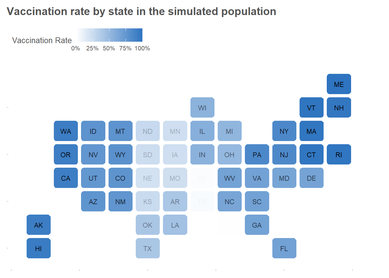
To make the example more interesting, we’ll divide the population into U.S. states with differing vaccination rates.
Show R code
pop$census_division <- cut(plogis(random_component + rnorm(N, 0, 1)), 9)
levels(pop$census_division) <- c("East South Central", "West North Central",
                                 "West South Central", "East North Central",
                                 "South Atlantic", "Mountain",
                                 "Middle Atlantic", "Pacific",
                                 "New England")
for (division in unique(pop$census_division)) {

  states_in_division <- state.name[state.division == division]

  for (i in which(pop$census_division == division)) {
    pop[i,'state'] <- sample(states_in_division, size = 1)
  }
}
Drawing a sample and estimating vaccination rates
Because we ultimately care about whether this method works for complex samples and not just simple random samples, we’ll draw a stratified multistage sample. Specifically, we’ll sample three states from each of the nine geographic Census divisions and then sample 100 people from each of the two sampled states.
library(survey)

# Draw a stratified multistage sample ----

  sample_data <- pop %>%
    # Sample two states from each census division
    group_by(census_division) %>%
    mutate(N_states = n_distinct(state)) %>%
    filter(state %in% sample(x = unique(state),
                             size = 3, replace = FALSE)) %>%
    # Calculate the first stage sampling probability
    mutate(stage_1_prob = 3/N_states) %>%
    # Sample 100 persons from each sampled state
    group_by(state) %>%
    mutate(N_in_State = n()) %>%
    sample_n(size = 100, replace = FALSE) %>%
    # Calculate the second stage sampling probability
    mutate(stage_2_prob = 100/N_in_State) %>%
    ungroup()

# Calculate weights ----

  sample_data <- sample_data %>%
    mutate(weights = 1 / (stage_1_prob * stage_2_prob))
Next we set up a survey design object using the survey package so that we can correctly estimate sampling variances.
# Set up a survey design object

  survey_design <- survey::svydesign(data = sample_data,
                                     weights = ~ weights,
                                     strata = ~ census_division,
                                     ids = ~ state    + Person,
                                     fpc = ~ N_states + N_in_State)
With this sample, we’ll estimate the vaccination rates using the svyratio() function. One of the benefits of using this function is that we can obtain the (estimated) influence functions for the two vaccination rates for all of our sample cases by specifying the option influence = TRUE. This is a nice option included with many functions in the survey package, such as svymean(), svytotal(), and even svyglm(), although it’s confusing because it doesn’t really return the influence functions but rather returns the influence functions multiplied by the weights.
# Estimate vaccination rates
# and retain (estimated) influence functions
  rate_30_to_50 <- survey::svyratio(numerator = ~ Vaxxed_30_to_50,
                                    denominator = ~ Aged_30_to_50,
                                    design = survey_design,
                                    influence = TRUE)
  rate_40_to_60 <- survey::svyratio(numerator = ~ Vaxxed_40_to_60,
                                    denominator = ~ Aged_40_to_60,
                                    design = survey_design,
                                    influence = TRUE)

# Obtain (estimated) influence functions for the sample
#     - Note that the survey package returns influence functions
#     - **divided by inclusion probabilities**
#     - and so to get actual influence functions
#     - you have to multiply output by inclusion probabilities

  infl_fn_30_to_50 <- attr(rate_30_to_50, 'influence') * survey_design$prob
  infl_fn_40_to_60 <- attr(rate_40_to_60, 'influence') * survey_design$prob
Using the influence functions
Next, we’ll add the influence functions as variables in the data so that we can estimate the population totals of the influence functions using the svytotal() function. Of course, we don’t really care at all what the estimated population totals are; we just want to estimate the sampling variance and covariance of these estimated totals.
# Get estimated totals of the influence functions
# as well as the variances and covariance of these estimated totals

survey_design$variables[['infl_fn_30_to_50']] <- infl_fn_30_to_50
survey_design$variables[['infl_fn_40_to_60']] <- infl_fn_40_to_60

infl_fn_totals <- svytotal(x = ~ infl_fn_30_to_50 + infl_fn_40_to_60,
                           design = survey_design)
We can now obtain the estimated variance-covariance matrix of these totals using the generic vcov() function. This is extremely helpful for complex designs: if we set up the survey design object appropriately, the survey package simply does the right thing to estimate this variance-covariance matrix.
vcov_of_estimated_rates <- vcov(infl_fn_totals)And because of the fact that we can approximate the variance-covariance matrix of a pair of statistics using the variance-covariance matrix of the estimated influence function totals, this matrix answers our key question. This variance-covariance matrix gives us the variance and covariance of the estimates of vaccination rates in the two overlapping populations.
                 infl_fn_30_to_50 infl_fn_40_to_60
infl_fn_30_to_50     1.245841e-04     6.313564e-05
infl_fn_40_to_60     6.313564e-05     1.165309e-04
Note that, as we would hope, the estimated variances match the variances obtained directly from svyratio(). The only difference is that all our work has paid off by giving us an estimate of the covariance, too.
vcov(rate_30_to_50) Vaxxed_30_to_50/Aged_30_to_50
Vaxxed_30_to_50/Aged_30_to_50 0.0001245841vcov(rate_40_to_60) Vaxxed_40_to_60/Aged_40_to_60
Vaxxed_40_to_60/Aged_40_to_60 0.0001165309For interpretability, we can convert this to a correlation matrix, which tells us that the two estimates have a strong correlation: \(\rho=0.52\). So it’s important to take this correlation into account if we want to estimate differences in vaccination rates between the two overlapping age groups.
cov2cor(vcov_of_estimated_rates) infl_fn_30_to_50 infl_fn_40_to_60
infl_fn_30_to_50 1.0000000 0.5239897
infl_fn_40_to_60 0.5239897 1.0000000Evaluating the method using simulations
In the example above, we were able to show that the influence function method gave correct variance estimates for the two vaccination rates. But how can we know whether it also gave a reasonable estimate of the covariance? We can use simulation to help us out.
We’ll simulate the sampling and estimation process 10,000 times. This lets us do two things:
- We can determine the “true” sampling covariance by calculating the covariance across all 10,000 samples
- We can compare the “true” sampling covariance to the distribution of estimated covariances obtained using the influence function method.
This whole process can be accomplished using the handy replicate() function and our previous code.
Show R code
# Set up parallel processing
# so we can use `future_replicate()`
# in place of the base function `replicate()`

library(future.apply)
plan(multisession(workers = availableCores() - 1))

# Simulate the sampling and estimation process 10,000 times

sim_output <- future_replicate(n = 10000, simplify = FALSE, expr = {

  # Draw a stratified multistage sample ----

    sample_data <- pop %>%
      # Sample two states from each census division
      group_by(census_division) %>%
      mutate(N_states = n_distinct(state)) %>%
      filter(state %in% sample(x = unique(state),
                               size = 3, replace = FALSE)) %>%
      # Calculate the first stage sampling probability
      mutate(stage_1_prob = 3/N_states) %>%
      # Sample 100 persons from each sampled state
      group_by(state) %>%
      mutate(N_in_State = n()) %>%
      sample_n(size = 100, replace = FALSE) %>%
      # Calculate the second stage sampling probability
      mutate(stage_2_prob = 100/N_in_State) %>%
      ungroup()

  # Calculate weights ----

    sample_data <- sample_data %>%
      mutate(weights = 1 / (stage_1_prob * stage_2_prob))

  # Set up a survey design object

    survey_design <- survey::svydesign(data = sample_data,
                                       weights = ~ weights,
                                       strata = ~ census_division,
                                       ids = ~ state    + Person,
                                       fpc = ~ N_states + N_in_State)
  # Estimate vaccination rates
  # and retain (estimated) influence functions

  rate_30_to_50 <- survey::svyratio(numerator = ~ Vaxxed_30_to_50,
                                    denominator = ~ Aged_30_to_50,
                                    design = survey_design,
                                    influence = TRUE)
  rate_40_to_60 <- survey::svyratio(numerator = ~ Vaxxed_40_to_60,
                                    denominator = ~ Aged_40_to_60,
                                    design = survey_design,
                                    influence = TRUE)

  # Obtain (estimated) influence functions for the sample

  infl_fn_30_to_50 <- attr(rate_30_to_50, 'influence') * survey_design$prob
  infl_fn_40_to_60 <- attr(rate_40_to_60, 'influence') * survey_design$prob

  survey_design$variables[['infl_fn_30_to_50']] <- infl_fn_30_to_50
  survey_design$variables[['infl_fn_40_to_60']] <- infl_fn_40_to_60

  # Get estimated totals of the influence functions
  # as well as the variances and covariance of these estimated totals

  infl_fn_totals <- svytotal(x = ~ infl_fn_30_to_50 + infl_fn_40_to_60,
                             design = survey_design)

  vcov_of_estimated_rates <- vcov(infl_fn_totals)

  # Collect output

  data.frame(
    'rate_30_to_50' = as.numeric(rate_30_to_50$ratio),
    'rate_40_to_60' = as.numeric(rate_40_to_60$ratio),
    'covariance_est' = vcov_of_estimated_rates['infl_fn_30_to_50','infl_fn_40_to_60'],
    'correlation_est' = cov2cor(vcov_of_estimated_rates)['infl_fn_30_to_50','infl_fn_40_to_60']
  )
})

sim_output <- Reduce(f = rbind, x = sim_output)
To get a sense of what the simulation output looks like, we’ll look at the first few rows of data, where each row includes the statistics estimated from a given sample.
  rate_30_to_50 rate_40_to_60 covariance_est correlation_est
1     0.6487634     0.7726384   6.000499e-05       0.4639787
2     0.6391239     0.7870213   5.262493e-05       0.4596900
3     0.6555370     0.7845107   7.905778e-05       0.5659938
4     0.6632941     0.8082116   5.441709e-05       0.3963841
5     0.6471729     0.7982499   5.774904e-05       0.4953169
With these statistics from the 10,000 simulated samples in hand, we can now get an empirical estimate of the “true” sampling correlation between the estimates for the two overlapping groups.
# Calculate covariance and correlation matrices
# of statistics across simulated samples
empirical_cov <- cov(sim_output[,c('rate_30_to_50', 'rate_40_to_60')])
empirical_corr <- cov2cor(empirical_cov)

# Pull the correlation and covariance from the matrices
empirical_cov <- empirical_cov['rate_30_to_50', 'rate_40_to_60']
empirical_corr <- empirical_corr['rate_30_to_50', 'rate_40_to_60']
This lets us estimate the bias and root mean square error of the correlation estimates:
empirical_bias <- mean(sim_output$correlation_est) - empirical_corr

print(empirical_bias)
[1] -0.009140477mse_corr <- mean(
(sim_output$correlation_est - empirical_corr)^2
)
rmse_corr <- sqrt(mse_corr)
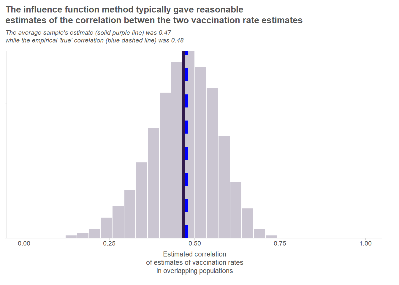
print(rmse_corr)[1] 0.1012603That’s pretty good! The method yields virtually unbiased estimates of the correlation, and the mean square error is pretty manageable. As we can see in the chart below, the estimates follow a nice bell-shaped curve around the empirical true correlation. All in all, the method seems to have resulted in reasonable estimates of the correlation between the two overlapping populations’ vaccination rates.
Footnotes
The population total of the influence functions, \(Z=\sum_{i \in U}z_i\), has no real meaning. We just care about the variance of the estimated population total, \(Var(\hat{Z})\).↩︎